TROID Classification is backed by Bayesian decision theory, which allows for expressing the probability of a particular class given an observed measurement x as:

P(Cj│x) = P(x,Cj)/P(x) = (P(x│Cj) P(Cj))/P(x)

where P (x, C_j) is the joint probability of  x and C_j, P (x | C_j) denotes the conditional probability of the data given the class. In order to establish a lithoclass (e.g., Gas Sand, Oil Sand, High-Resistivity Reservoir, or Shale), a rock diagnostic is performed where a set of crossplots is generated utilizing petrophysical logs and inversion output attributes. The objective is to determine which attributes best separate the desired lithoclasses in the multidimensional data space.

The Gaussian Mixture Model (GMM) Advantage

Our classification workflow utilizes the Gaussian Mixture Model (GMM) to define the probability density functions (PDFs). Unlike simpler methods that treat logs as independent, GMM accounts for the physical correlation between measurements—mathematically capturing the “handshake” between different rock properties.

I. Establishing the Statistical Territory

In the analysis below, we utilized Z-score standardized gamma ray and neutron logs to differentiate between High-Resistivity (High_RES) and Low-Resistivity (Low_RES) facies.

• The Tilted Ellipses: The 2σ ellipses represent the model’s territory for each facies, capturing approximately 95% of the data for that specific rock type.

• Modeling Correlation: The “tilt” of the ellipses proves the model is correctly accounting for the covariance between Gamma and Neutron, leading to a more robust separation than standard cut-offs.

II. Validation and Performance Metrics

To ensure the reliability of the Bayesian posterior probabilities, we validate the model using a confusion matrix. In our recent multi-well study, the model demonstrated exceptional performance within the analysis window.

• 94.3% Overall Accuracy: Out of 1,414 total samples, the model correctly identified the facies in 1,334 instances.

• High Reservoir Recall: The model successfully “caught” 96.0% of all actual High-Resistivity zones, minimizing the risk of missing potential pay.

Rigorous Framework

These probability density functions (PDFs) are ultimately applied to selected seismic inversion or machine learning inversion outputs to produce class and probability volumes. At each sample, the associated probability represents the likelihood of each class defined based on the crossplot analysis.

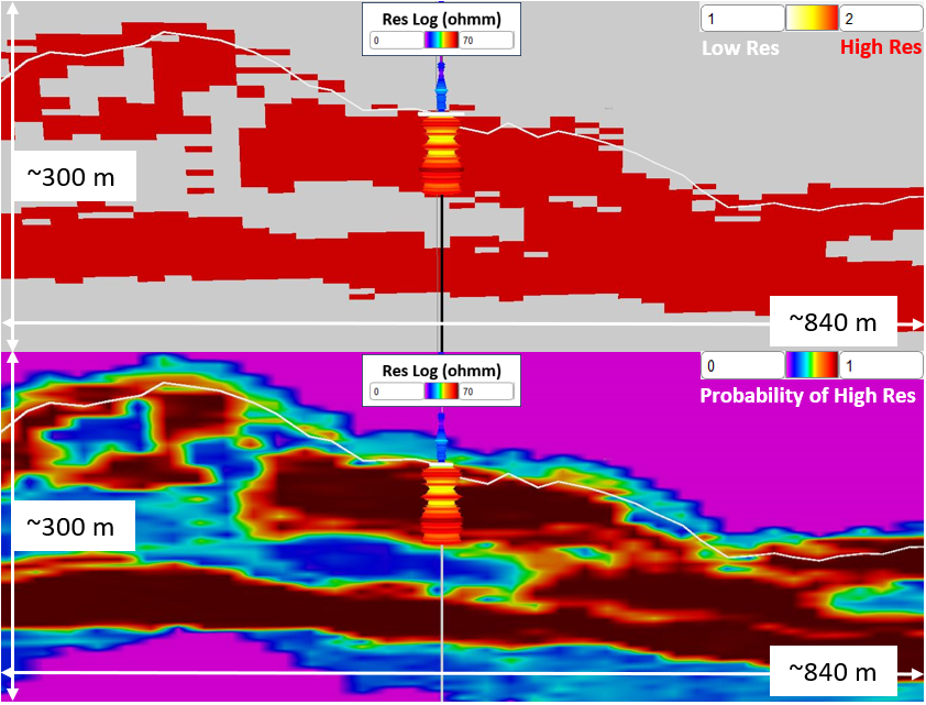
The results produced from a High Res and Low Res facies prediction study are shown below.  The top figure shows the predicted facies where red corresponds to High Res and gray is Low Res. The lower figure is the associated probability of the High Res facies. The resistivity well log is shown with a range of 0-70 ohmm. This results shows a high correlation between the facies prediction and the kick in high resistivity observed at the well. The well marker and interpreted seismic horizon are also displayed.

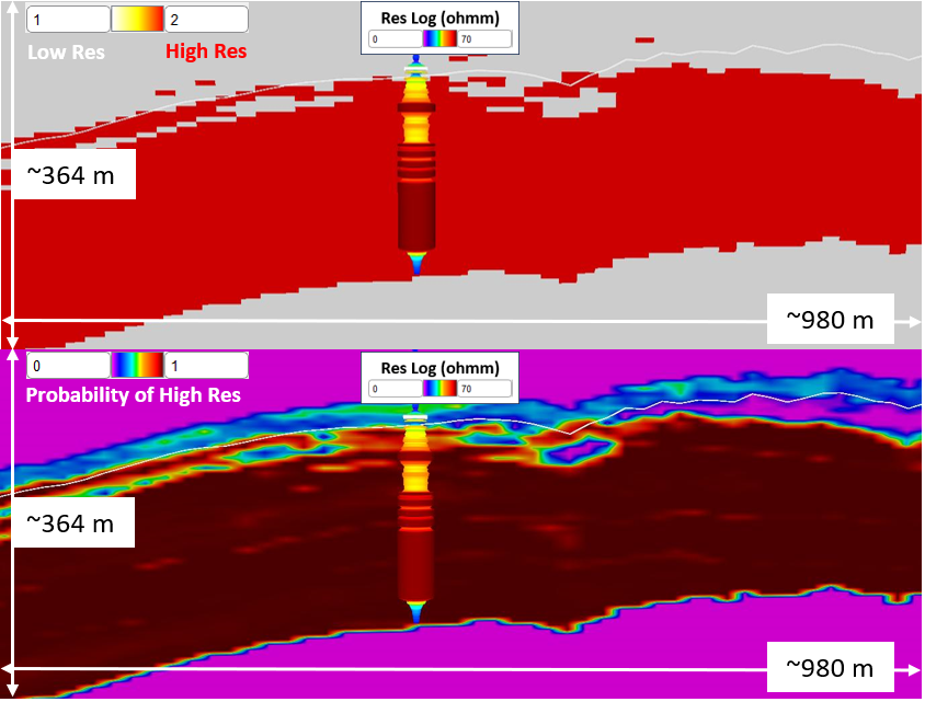
The next figure show the result at a well that was not used in the classification analysis nor the low frequency model in the machine learning inversion carried out prior to Bayesian classification (blind well). The location of this well is two kilometers from the previous well shown. The prediction shows a high correlation with the resistivity increase in the well log.